When Petri-nets were introduced to me, they were being described explicitly as a type of model that is not Turing-complete. While this might be true, I will prove in this article that a slightly generalized form of Petri-nets which allows for infinitely many places and infinitely many transitions is Turing-complete. After, I will show that normal Petri-nets (with finite places and transitions) can be used to implement any total Turing machine (a.k.a. decider, i.e. a machine that halts for every input), which are not as powerful as general Turing machines but still have more computational power than real computers. This also implies that Petri-nets can be used to decide any recursive language.

To prove this, I will first introduce a machine design for simulating Turing machines with generalized Petri-nets, and afterwards modify this machine design to suit the restrictions of normal Petri-nets. My previous article on Boolean pairs is a prerequisite for this article, because I will be using Boolean pairs in the machine design.

It has previously been proven that Petri-nets with some types of non-standard features are Turing-complete (such as inhibitor arcs (Agerwala 1974)). In this article I will only be using standard Petri-net functionality. As a matter of fact, this proof is also valid for a more restrictive version of Petri-nets where no place may ever contain more than one token.

to prove the Turing-completeness of slightly generalized Petri-nets (which are allowed to have infinite places and transitions)

Finite and infinite Petri-nets

The machine design which I will provide cannot be built in a normal Petri-net. This is because a Turing machine must have an infinitely long tape (or a limitlessly growing tape), and the machine design uses an infinite amount of places and transitions for its infinitely long tape. Strictly by the definition of Petri-nets, the amount of places and transitions must be finite (Peterson 1981), so this is not possible for normal Petri-nets. For this reason, I will first be proving the Turing-completeness of a slightly generalized form of Petri-nets, which doesn’t have the constraint that the amount of places and transitions must be finite, and then deriving a modified machine design which can be used to decide recursive languages with a normal (finite) Petri-net.

Despite the fact that the Turing-completeness proof does not apply directly to normal Petri-nets, I wish to note that it does show that normal Petri-nets are very, very close to being Turing-complete, as it shows that a modeling language with all the important mechanisms of a Petri-net is Turing-complete. It is only the constraint that a Petri-net must be finite which saves it from being theoretically Turing-complete.

Furthermore, even though Petri-nets technically might not be Turing-complete, I think it can nonetheless be productive to think of Petri-nets as being “as good as Turing-complete for practical purposes”, because any computation that does not strictly require infinite memory can be performed on a finite-size Petri-net, and any computation that we use in practice does not require infinite memory.

Anyhow, let’s move on to the machine design.

Machine design

The machine design is too complex to show it in its entirety in one image. Instead, I will be showing the machine design in parts. I have given certain places a name and these places will reappear in various diagrams — each time representing the exact same place.

I wish to note that I will be slightly informal throughout this section, because I believe being perfectly formal can get in the way of getting the message across clearly. One such informality is that I have chosen to show a machine which will use exactly three boolean pairs to encode a symbol, and therefore it can only have up to eight different symbols (counting blank as one of the symbols). However, I will be using designs that are quite easy to extend to use a larger amount of boolean pairs per symbol, thereby allowing for more symbols. I have made the decision to always show cells consisting of three boolean pairs purely to make the diagrams more simple.

Overview without transitions

First, let us look at an overview of only the important components of this machine design. Transitions are not included in this overview and many places have been left out. Collections of boolean pairs that together represent a symbol have a rounded rectangle drawn around them.

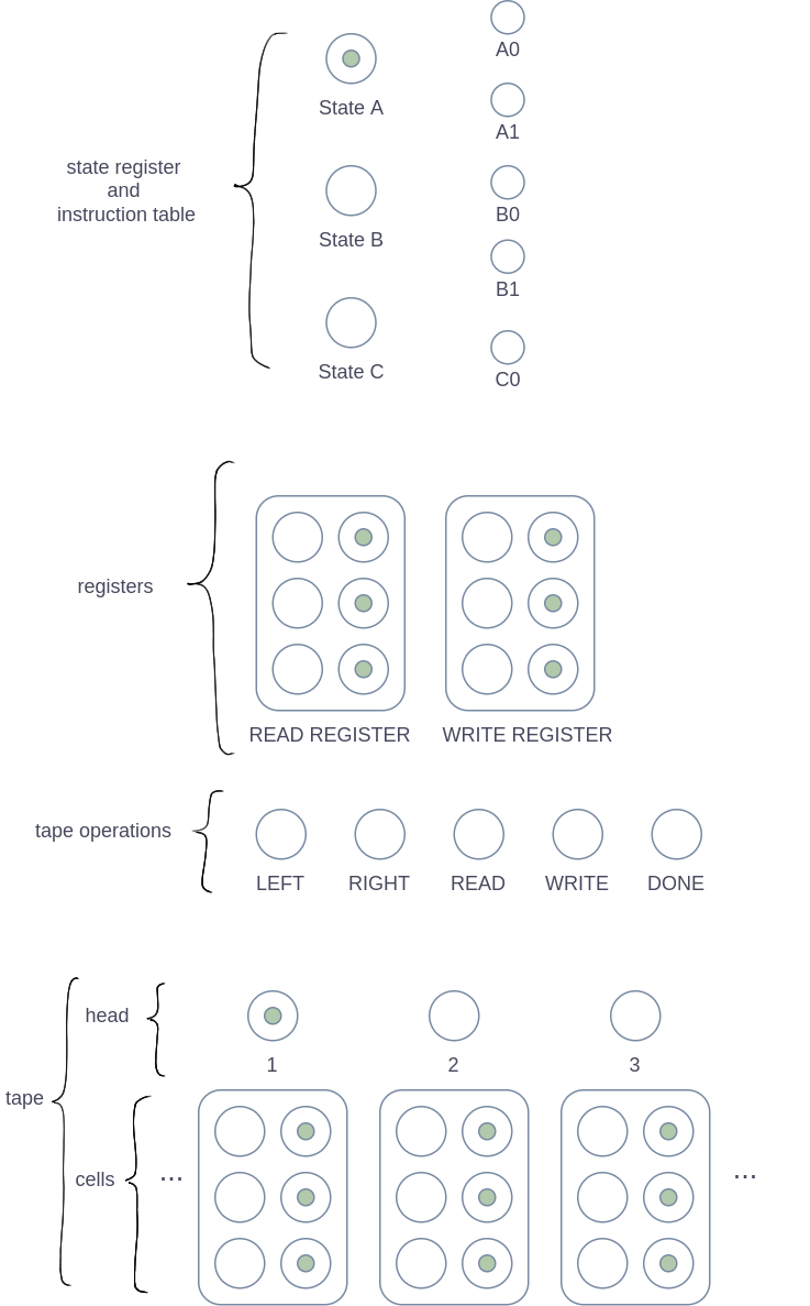
In this overview I have shown a machine with three states and five instructions total, but this machine design can easily be generalized to other amounts of states and instructions. Most of the places in the state register and instruction table have not been included, but they will be shown in a later section. For now, it suffices to say that each state has a “starting place”, labelled “State A”, “State B” and “State C”, and each state has an amount of instructions, which are labelled “A0”, “A1”, and so on. The naming convention I have used for instructions is that the letter indicates the state and the number indicates the (decoded) scanned symbol necessary for that instruction.

Below the state register and the instruction table, you can see a pair of registers. These registers aren’t strictly necessary — it is possible to remove them from the machine design entirely —, but they help to reduce the complexity of the design. For each instruction, the contents of the cell under the head are copied to the read register by the READ tape operation, and later the contents of the write register are copied back to the cell under the head by the WRITE tape operation. Thanks to this, the instructions only need to manipulate the registers in different ways. It would be relatively complicated if instructions needed to manipulate the cells on the tape directly.

There are four tape operations, which can be started by putting a token into one of the LEFT/RIGHT/READ/WRITE places. The tape operations are as follows:

• LEFT: Move the head one cell to the left
• RIGHT: Move the head one cell to the right
• READ: Copy the contents of the cell under the head to the READ REGISTER
• WRITE: Copy the contents of the WRITE REGISTER to the cell under the head

After starting a tape operation, the environment from where it was started should wait until the tape operation finishes. For this purpose there is a special DONE place, which gets a token after a tape operation finishes. Only one tape operation may be executed at once.

The tape consists of an infinite amount of cells, which is depicted somewhat informally in the diagram with only three cells and ellipses on either side. In a standard Turing machine the tape extends infinitely to the left as well as to the right, so in this machine the tape also extends infinitely in both directions. Notably it is not actually necessary for the tape to extend infinitely in both directions. After all, Turing’s original a-machine model had a tape that only extended infinitely in one direction and not in both. Nonetheless, the decision was made to extend it infinitely in both directions because this seems to be considered standard for a Turing machine nowadays.

Any binary encoding will work for storing symbols in the cells. I have used binary counting, with the lowest boolean pair in the diagrams being the least significant binary digit. In the overview diagram, all cells contain the blank symbol, encoded as zero.

In a Turing machine, the head indicates which cell is currently being manipulated. In this machine design, each cell on the tape is accompanied by a place which is used to keep track of the position of the head. When this place has a token, the head is at that cell. This means that only one place out of all head places should have a token at a given moment. In the overview diagram, the head is at cell 1.

Having had a look at the overview, we will now look at the components in more detail. First we will look at the implementation of each of the tape operations. Afterwards we will look at how states and transitions work. However, before we can get to tape operations, we need to look at the most important operation that we will perform on cells: copying.

Copying symbols

In this section, I will discuss the implementation of the most important operation that we will use on cells: Copying the contents of a cell to another (of course, overwriting the other cell in the process). This section contains the most convoluted diagram of this entire article, so as to make the diagrams of the rest of this article less complex, I will also introduce a simplified notation specifically for copying.

The diagram below contains an implementation for copying the symbol in the SOURCE cell to the DESTINATION cell. This implementation is specifically for cells consisting of three boolean pairs, but the operation goes through the cells boolean-by-boolean doing the exact same operation for each boolean pair and can therefore easily be extended for machines which need more than eight symbols.

For visual clarity, arrows are categorized and colored in the diagram: Blue arrows indicate control flow, green arrows indicate a data check and yellow arrows indicate data manipulation. I have put a token in the START place so that you can try executing the copy operation in your head.

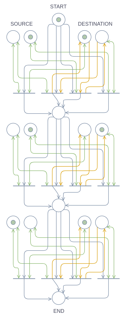
Essentially this implementation goes through the boolean pairs in the destination cell and checks if it’s the same as the corresponding boolean pair in the source cell. If the boolean pair in the destination cell is already the same as the boolean pair in the source cell, it doesn’t need to be changed. Otherwise, the boolean pair in the destination cell gets its value flipped.

It is not actually necessary to copy boolean-by-boolean. We could also copy the contents of one cell to another in just one step, but it would take a very large amount of transitions. Moreover, the depicted implementation scales up for machines with more boolean pairs per cell quite nicely.

I will use the copy operation in three out of six remaining diagrams, so I’ve given it a special simplified notation, which can be seen in the image below:

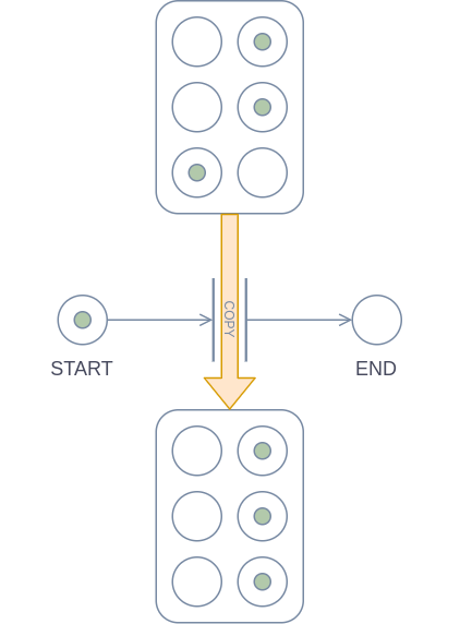
The fat arrow indicates which cell is being copied to which other cell, with the cell at the head of the arrow of course being the destination. Any appearance of this notation can be substituted by the lengthier implementation from before. Notably this notation is only for convenience and does not increase the power of Petri-nets (since, as I said, it can be substituted by the full implementation).

Tape operations

LEFT & RIGHT

The LEFT and RIGHT operations are quite simple: We add a transition for each pair of subsequent head places, and when the head token is currently in the first of these places, we take it away from there and move it into the second place. The only difference between these two operations is the direction of the arrows between the head nodes and the transition.

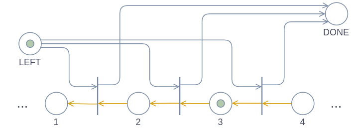
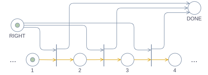
Both of the diagrams above will end with the head node being at cell 2.

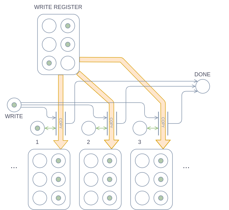
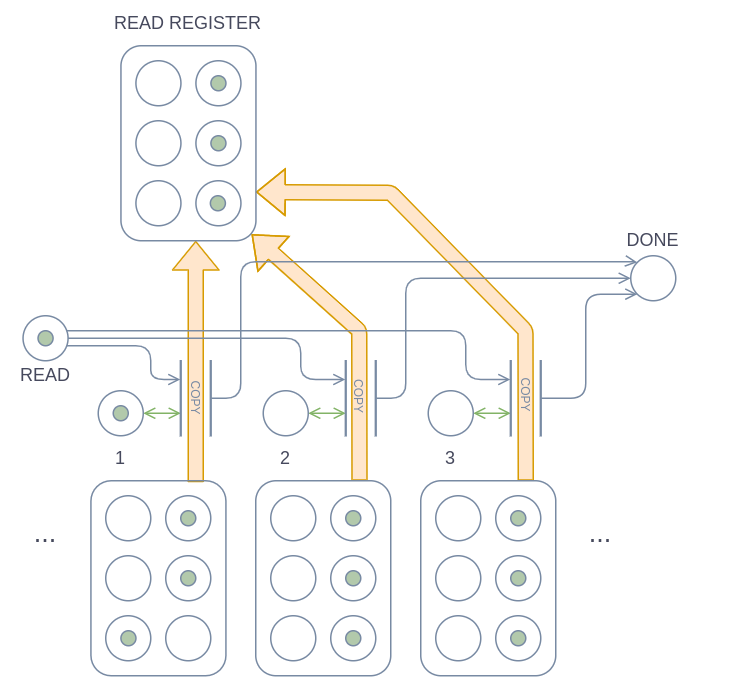
READ & WRITE

The WRITE and READ operations are also quite similar to each other. Thanks to the special notation for copying, the implementation is quite simple.

During a WRITE operation, the WRITE REGISTER is copied to a specific cell on the tape if the WRITE place has a token and the cell’s head place has a token. After the copy operation is finished, the DONE place gets a token. The READ operation works the same as WRITE, except that it copies from the cell to the READ REGISTER instead of the other way around.

State register and instruction table

The state register and instruction table are the only parts of this machine design that need to be changed to simulate a different Turing machine (unless you want more than eight different symbols, then the tape and registers would need to be changed). It is important to note that this machine design is not inherently a universal Turing machine, and therefore it does need more changes than just different inputs to simulate a different Turing machine. States

A Turing machine can have any finite number of states. Each state has a finite number of instructions associated with it, and which instruction is performed depends on which symbol is currently under the head of the tape.

Below you can see the implementation of an example state X. This state has two instructions, X0 and X1, which are executed when the scanned symbol is either 0 (false-false-false) or 1 (false-false-true) respectively.

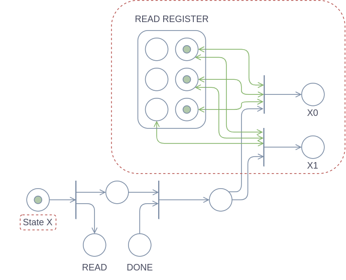
In steps:

• The state starts when a token is in the “State X” place
• Then, we start a READ operation. We use a special waiting place so that we can recontinue where we left of when the DONE token comes in.
• Then, we check which symbol was placed in the READ REGISTER by the READ operation. In this case we check for 0 or 1. If any other symbol is in the READ REGISTER, the machine will halt.
• We then give a token to one of the instructions, depending on which symbol was found.

The parts of this component that will differ between different states and machines are outlined with a red dashed line:

• The name of the state can change.
• The instructions and which symbols they require can change.

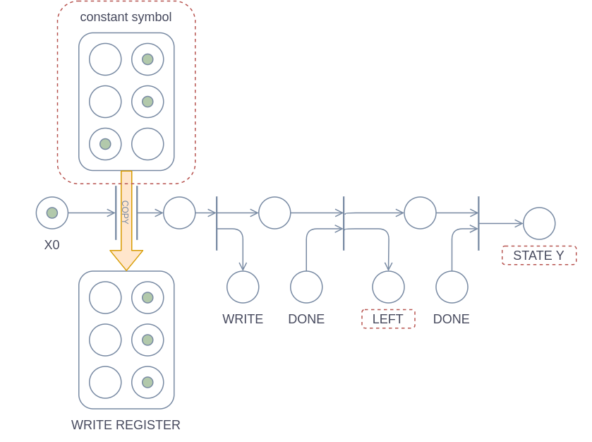
Instructions

In a Turing machine, an instruction does three things: It writes a symbol to the cell under the head, it moves the head left or right, and then it goes to the next state. It differs between instructions which symbol is written, which direction the head moves towards and which state we go to next.

The Petri-net implementation of this can be seen below. This uses mostly the same techniques as were used for implementing states. The instruction in the diagram writes the symbol 1 (false-false-true), moves the head left and goes to state Y.

That concludes the machine design. Put all of these parts together and you will have a full-fledged Turing machine for slightly generalized Petri-nets. For normal Petri-nets, however, getting an infinitely large tape may prove impossible.

Implications for normal Petri-nets

Normal (finite) Petri nets are not Turing-complete, as was proven by Agerwala (1973). Nevertheless, if one were to try to create as powerful a machine as possible with only a Petri-net with a finite amount of places and transitions, then Petri-nets are still sufficient to simulate any total Turing machine. Notably, a total Turing machine is not the same as a normal “general” Turing machine. Total Turing machines have the additional restriction that the machine must always halt eventually. This makes them slightly less powerful than general Turing machines, but still powerful enough to decide recursive languages.

Modifying the previous machine design to simulate only total Turing machines is almost trivial: Instead of having an infinitely long tape, the length of the tape is constrained to some function of the length of the input. Notably, this can be any function and not just a linear function. If the function could only be a linear function, this modified machine design would be a linear-bounded automaton, which is less powerful than a total Turing machine. In this situation, we are not constrained to only using a linear function for the length of the tape, and because of this, the new machine design can simulate all total Turing machines.

The fact that this modified machine design can simulate any total Turing machine is not entirely trivial, so I will take a moment to explain. A total Turing machine is a type of Turing machine that is known to halt eventually, which means that it halts within a finite amount of steps. In a finite amount of steps, the tape’s head can only be moved a finite amount of cells. If you give a total Turing machine every possible input of a specific size, all of the executions of the machine will, of course, end in a finite amount of steps. To be able to simulate all of those executions on a machine with a limited amount of tape, the machine’s tape only needs to be longer than the largest amount of steps that any of the executions will take before halting (although both to the right and to the left, so really, it needs to be at least twice as long as the largest amount of steps). This means that the tape would be so long, that none of the executions would run for long enough to be able to get past the ends of the tape. Therefore, given a certain total Turing machine and a certain input length n, there is always a tape length above which the modified machine design can fully simulate the total Turing machine for every input with the length n. Furthermore, the modified machine design can simulate a total Turing machine with an input of any length as long as the function that determines the length of the tape is chosen well, so that the tape is always longer than the amount of cells the machine will be able to use.

The above is sufficient to conclude that the modified machine design is capable of simulating any total Turing machine, and that it can therefore decide any recursive language. More importantly, because the tape of this modified machine design is not infinite, it’s possible to build it in a normal Petri-net, and therefore Petri-nets in general must be at least as powerful as this modified machine design.

In conclusion, normal Petri-nets can decide recursive languages, and if Petri-nets were allowed to be infinitely large, they would be Turing-complete.

References

• T. Agerwala, “Comments on capabilities, limitations and “correctness” of Petri nets”, 1973.
• T. Agerwala, “A complete model for representing the coordination of asynchronous processes”, 1974.
• J. Peterson, “Petri Net Theory and the Modeling of Systems”, 1981